Amortization Tables Explained

Amortization tables are commonly used in the financial sector. They list out the periodic payments on a loan or mortgage over a period of time and break down each payment into principal and interest. When we create an amortization table in Excel we can define, the amount we are borrowing, the interest rate, the number of payments, if we are paying at the beginning or end of the month, the start date, and if we have a balloon payment to clear the balance.

Creating an Amortization Table

• Go to the File tab.
• Click on the New page.
• Type "amortization" into the search bar.

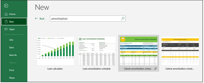
In this example, we are going to start from a blank template that does not contain any formulas.

Understanding the Amortization Schedule

Before we start adding calculations and formulas, let's first understand what we are looking at.
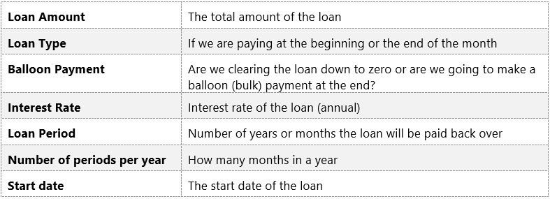
At the top, we have the details we need to calculate the monthly payments on a loan.

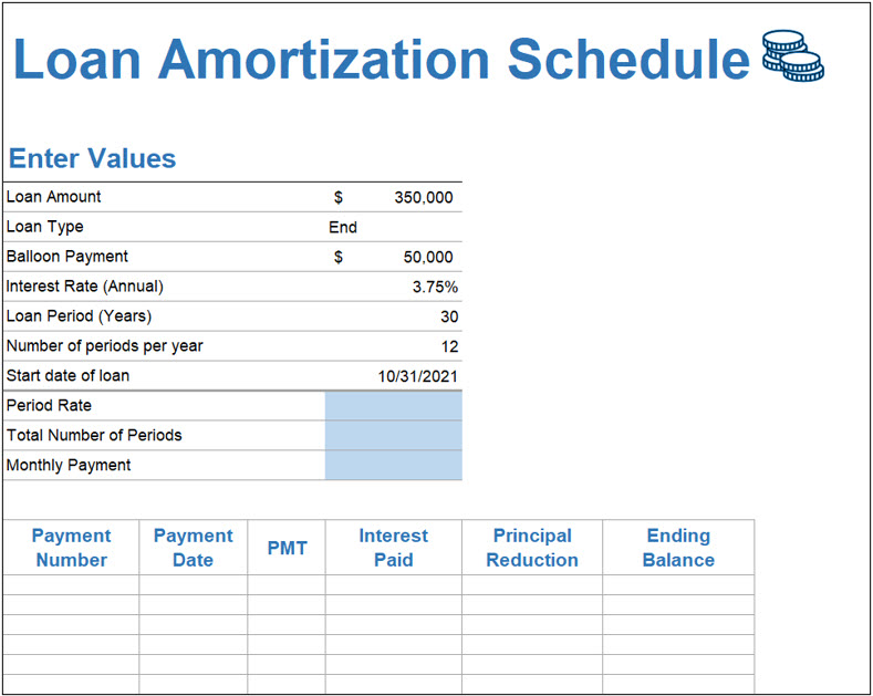
In this example, we are borrowing $350,000 to buy a house. We have $50,000 in savings which we will use at the end of the loan to clear the balance.

To calculate our monthly payments over the term of the loan, we need to first use formulas to work out the Period Rate, the Total Number of Periods, and the Monthly Payment. Once we have these calculations, we can use them to complete the amortization table.

Calculating the Monthly Payment

• Type =SUM(D9/D11)

We are paying a monthly interest rate of 0.31250%.

Total Number of Periods

• Type =SUM(D10*D11)

The loan will be paid over a total of 360 months.

We can now use the PMT function in Excel to calculate the monthly payment. PMT stands for Payment and it is one of Excel's Financial functions.

This is how our PMT formula looks. Note the highlighted cells used in the calculation.

The PMT formula will produce a negative result by default. This is because Excel sees this money as being taken from your account.
To make this a positive value, press F2 to edit the PMT formula and add a minus sign before the pv.

The total monthly payment for this loan is $1,545.60.

We can now use the monthly payment to complete the amortization table.

Completing the Amortization Table

An amortization table allows us to see how much interest we are paying and how much the principal amount decreases by over the period of the loan. We need to complete each column in the table.

Payment Number

• Type 0 into the first cell.
• Hold down the right mouse button, drag the fill handle down one cell and then back up one cell to reveal a secret menu.
• Select Series from the menu.
• In the Series in area, select Columns.
• Add a Stop value of 360.

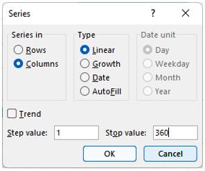
• Click OK.

Payment Date

• Manually type the date of the first payment in the cell next to payment 1.
• Double-click the fill handle to fill the dates down.

• Click the Autofill Options button.
• Select Fill Months from the menu.

The dates will now be the last day of every month.

PMT

• Double-click the fill handle to copy the formula down.

Interest Paid

Next, we need to calculate the amount of interest paid each month. This will change as the loan reduces. To make this easier, we are going to add the Ending Balance in the first row of the table.

• Click in Interest Paid.

The Interest Paid is the Balance * Monthly Interest Rate. We are going to copy this formula down so remember to lock cell D13. This calculation tells us how much interest we will pay each month.

Principal Reduction

Next, we need to calculate the Principal Reduction. This is the amount we are paying on the balance of the loan that is not interest. This is a simple calculation of PMT - Interest Paid. 

Ending Balance

Finally, we need to calculate the Ending Balance. This is the amount outstanding on the loan each month. This is a simple calculation of Ending Balance - Principal Reduction.

Completing the Amortization Table

• Select all cells in the second row that contain calculations.
• Double-click on the fill handle to copy down.

If the amortization table has been completed correctly, we should see that payment 360 has an ending balance of $50,000. It is at this point we would make our balloon payment to clear the loan.

Notice that as the loan reduces the amount of interest we are paying also reduces and the amount we are paying off the principal increases.

Rounding

When working with financial spreadsheets and money, we need to be as accurate as possible. If we apply rounding to our amortization table, the ending balance will be a few pennies off but the calculations will be more accurate.

To round all calculations in the amortization table, we only need to round the PMT formula and the Interest Paid formula.

• Press F2 to edit the PMT formula.
• Round the result to 2 digits.

• Press F2 to edit the Interest Paid formula.
• Round the result to 2 digits.
• Copy the formula down using the fill handle.

For additional information on this topic in the MMC course library, check out all our Excel courses.